This sample example explains how primary particle composition and flux are defined in the ‘primary’ file.
In this sample COSMOS simulation ONLY outputs primary information at the beginning of each event
(primary injection) and exits without any air shower production.
Output file can be converted into the spectra by a ROOT script so that we can confirm if the spectra
are as expected.
make clean; make
./cosmosMacGfort < param > out 2> err # (here 'MacGfort' depends on your system.)
root primary_analysis.cpp # (assuming you can use ROOT.)
Particles are injected from 100km (100e3 meters) above the sea level and the obsevation site
is defined at 99km. So there is essentially no interaction.
Usually DepthList is used to define the obsevation height in kg/m^2 and HeightList in meter is
calculated inside COSMOS.
However, if it is defined in negative value like this sampe, HeightList is referred and DepthList
is calculated.
DestEventNo = 100000
100k primary particles are injected.
Because we do not simulate air shower, it is done in O(10sec).
chook.f contained user subroutines where the users can define actions at each process of simulation.
In this sample, except chookBgEvent subroutine, nothing is done.
You can confirm the subroutines are empty.
The subroutine chookBgEvent is called when a new injection particle is defined.
In this sample in chookBgEvent, the information (particle code etc) are printed to the standard
output. Immediately after that, all information in the particle stack is cleaered using
call cinitStack
so that simulation of this event terminates. (It does not track down to 99km as explained above.)
This example shows how to set electric/magnetic field.
Electric field is controlled by the parameter, HowEfield in &HPARAM,
which is 0 (disabled) by default.
Note that dielectric breakdown is not taken into consideration
even if very strong electric field is defined.
Magnetic field is controlled by the parameter, HowGeomag in &HPARAM,
which is 11 (constant geomagnetic field calculated at BaseL) by default.
Scrpt/CompileExampleByCMake.sh Application/Example/MyField
cd Application/Example/MyField
./cosmosLinuxGfort < param out 2> err
 # here 'LinuxGfort' might be different depending on your system
 # For 'param' file, see below.
 # trace1 will be generated.
ReadTraceMacro.C can be used in the directory to show the trace file
for param-e1 and param-e2.
For param-b1, the macro in the FirstKiss example will be used.
3 different param files are given.
For param-e1 and param-e2, primary_e (50GeV electron) will be read as primary and for param-b1, param_n (100GeV/n Nitrogen) will be read.
param-e1HowEfield=1 is set.
User can define upto 5 layers with constant electric fields
by parameters myEf(i)%H1, myEf(i)%H2, and myEf(i)%Ef in &HPARAM.
param-e2HowEfield=2 is set.
User defined subroutine, cmyEfield, will be called to calculate
the electric field at any place.
param-b1HowGeomag=22 is set.
In this example, the magnetic field exists at any place and the field
is the constant defined by the parameters (MagN, MagE, MagD) in &HPARAM.
(MagN, MagE`,``MagD) are North, East and Down components
of the magnetic field in the unit of Tesla in the detector system at BaseL.
This file is not specific to this example (electric/magnetic field).
To show the area where the electric field is not zero,
subroutine cmyTracePlus is called to show several layers of square
in the trace file.
In this example, artifitial electric field along z-axis
in the detector system is defined at x,y>0.
The z component of the field strength is calculated by:
where h is height [m].
In the param-e file, the primary will be injected with zenith angle >0.
The particle enters into the region where the electric field is finite
in the way of shower development and generate additional cascade
by the field.
Upgoing primary (e.g, tau lepton generated UHE nue inside earth)
We assume tau- or tau+ lepton which goes up from the surface area
of the Earth. For tau > 10^15 eV is interesting but we here
consider ~10TeV tau for quick calculation.
If Trace > 0 is given, the cmyTracePlus routine is called inside chookBgEvent in chook.f; it wrties a fake trace data at every observation depth.
The trace data is by a virtual heavy ion of negative charge and drwan with a white square line; its center is the 1ry axis position at the observation depth.
The default size is 6km x 6km. To omit the square, comment out the
callcmyTracePlus in chook.f. To modify the number of squares or to chage the shape, etc, modified cmyTracePlus.f. (Need not to add #include or similar action.)
It is included by #include in the cmain.f in Cosmos/cosmos; cmyTracePlus.f in the prsent directory has priority.
(See last few slides in FigA.pdf and the comment in cmhyTracePlus.f).
The stuff here is to get information of multi-particle production by
high energy hadron inelastic collisions; (the information is the one
contained in “ptcl”; particle kind, momentum etc)
Similar information can be obtained by using Cosmos/Util/Gencol, but
there is some difference:
we can use a compound target such as PWO, Air (however note for dpmjet3) etc.
the program gives only produced particle information (/ptcl/ info.)
so we cannot know diffraction information. (Probably, possible to know it, if getDiffCode.f and Zintmodel.h are imported from Gencol).
One strange and interesting case is that Gencol cannot be used
for K0l/K0s incident with the dpmjet3 interaction model; in that case, we get
a message,”pdf is not ready for this projectile” (pdf: parton distribution
function).
But using this, we can get result for that case (results seems to be OK;
comparison with results by other models indicating so).
In param, you must set
For $PARAM
Freec=fIntModel='"epos"'! as you likeLatitOfSite=-90.,LongitOfSite=0.,CosZenith=(1.0,1.0).HeightOfInj=5100.or 4500.DestEventNo=500000000,500000000! large number
For $HPARAM
UserHooki=1,100! output type & actual # of events to be generatedreadymadeoutputtype is oneof0,1,2:seelaterDpmFile="dpmjet.inp"! if target is air, comment out this! if target is non air and model is dpmjet3! use this; see later for dpmjet.inp.AtmosFile="Air+solid.d"! this is "atmosphere" with Air + Solid medium
--------
The target can be Air or another simple  nucleus (Fe, Pb...) or compound
nuclei (PWO etc).
For that  we
use  Air+Solid.d   as the "Atmosphere":
#-----------------------------------------------------------------
      4000    260.            0.80     Pb
      5000    250.            0.50     Air
To specify that the target is air, we must give injection height
h >= 5000.
To Specify Pb as the taget , 4000<=h <5000. If you replace Pb by PWO
the target will be PWO. The actual nucleus is randomly seleccted
with the weight of cross-section and number density of the nucleus.
NOTE: In the case of IntModel='"dpmjet3"', to use , e.g, Pb target,
the user must activate dpmjet.inp by DpmFile="dpmjet.inp"
and adjust the content of dpmjet.inp by giving the following 3:
PROJPAR
TARPAR
ENERGY
Two energy terms should be larger than the one in primary file.
(1st < 2nd one is better).
However, PWO like compound case cannot be managed by this way.
We must make dpmjet.inp (diff. from the we have been treating)
and dpmjet.GLB files. How to make such dpmjet.inp and dpmjet.GLB
will be given somewhere in LibLoft/Util/
Incident particle may be set by primary file.
3) Output type by UserHooki. The first value of UserHooki
fix the output type. See subroutine chookNEPInt in chook.f
The aim is to perform Monte Carlo simulations in a non-Earth environment, using the Sun as an example.
First, basic data representing the Sun should be prepared. The variables should be named the same as for Earth, but with values appropriate for the Sun. The data should be stored in a file named SunDef.d, although the name can be chosen freely. The file with the red text name should be located in the Sun folder.
The data should be recorded in a namelist named &ObjParam in the file mentioned above (the namelist name ObjParam is fixed). The values for Earth can be used as a reference and should be mentioned in the comments. Most of the data does not need to be extremely precise.
The structure of the solar atmosphere is included in SunAtmos.d, which can also be given a freely chosen name. As the composition differs from the Earth’s atmosphere, the sunAir defined as $LIBLOFT/Data/Media/sunAir should be used [1] .
Currently, the library uses the standard Earth atmosphere as the default option, but you can use the NRL Earth atmosphere, which depends on time and location, or a special atmosphere like the solar atmosphere. You can check which option is being used by running the atmosModel.sh command. If you want to change the atmosphere model, also use this command.
Coordinate systems
or the Sun, use the same coordinate system as for the Earth. Consider the Sun as a sphere and take the center as the origin of the E-xyz system. The x, y, and z axes can be determined appropriately depending on the problem. Longitude and latitude are also determined accordingly. The detector and primary systems can be determined in the same way.
When you create and run the program, a trace file is generated. You may expect to see an image like a cascade in the Earth’s atmosphere, but the solar atmosphere is so rarefied that there is little cascade development. You will likely see only a small number of particles spiraling in the magnetic field. Only about 10 to 20 out of hundreds of events will produce visually appealing images.
If you output trace data in the E-xyz system, you must output it in double precision; otherwise, the accuracy will be insufficient to produce correct drawings. If the drawing system is performing calculations in single precision, even with double precision output, the same will hold true (for example, in the Geomview case, the two .png files starting with Exyz in the Fig folder). In other cases, verb|Trace=1| is used with the primary system.
If BaseM doesn’t exist, proceed to create it and the following steps.
BaseM: It would be good to create new data with a new name by referring to Air in LibLoft/Data/BaseM. You don’t need to create it in BaseM at this stage, but eventually, it should be put in BaseM.
The value 29.0 in the middle is the molar mass – molecular weight (in /Mol or g/Mol units) for gases, so make sure to enter it.
Decompose the molecule into atoms, enter A and Z, and enter the relative abundance N. The ratio only needs to be relative.
The value at the bottom can be found by referring to the PDG’s web page in the following order:
PDG Web Page
Reviews, Tables & Plots
Atomic and Nuclear Properties of Materials (rev.) Interactive version
Select Interactive Version
Click on Inorganic compounds (Al through Fe) under the Periodic Table
...
Click on Mixtures
...
Find the relevant substance.
If there is one, select TEXT from the Table of muon dE/dx and Range: PDF TEXT
The row with values like this should appear at the top of the resulting table:

Sternheimer coef: a k=m_s x_0 x_1 I[eV] Cbar delta0
                 0.1091 3.3994 1.7418 4.2759 85.7 10.5961 0.00
Enter those values. If the substance cannot be found, enter -100.
Create Media Table Using the BaseM created above, create Sampling Tables, etc.
Go to LibLoft/Util/Elemag/BremPair.
Read the Readme file.
Run the following command:
Tables can also be created by calling other commands from this command. For example, for Air:
Air
Air.xcom
Furthermore, create:
Air.GLB
Air.inp
These are necessary for the hadron interaction of dpmjet3. To create them, execute the iniGlauber command without variables, find out how to use it, and execute it.
The five resulting files should be placed in LibLoft/Data/Media.
Sampling Test To test the Sampling Table created above, refer to item 2) of Readme in BremPair.
To learn about Hybrid AS calculation, handling magnetic pair creation, and various coordinate systems. Also, to understand how to obtain information when interactions occur.
chook.f, param, primary to be used: Each has a suffix of -XXX (XXX represents BfieldLine, etc. ). Use the same XXX for compiling and execution. Let’s summarize the types and meanings of XXX.
XXX
Purpose/Description
BfieldLine
Drawing magnetic field lines
Mag
Interaction between UHE-gamma and magnetic field
sync
Studying synchrotron radiation effects
Bounce
Drift and reflection of charged particles due to magnetic field
Once you have decided the XXX you want to try, remove chook.f using rm chook.f, then create a symbolic link by executing the command:
ln -s chook.f-XXX chook.f
After that, use
make clean; make
to create an executable binary (cosmos…). To execute it, use the command:
./cosmos... < param-XXX > outputfile 2> errorfile
The primary-XXX file is used for sampling the 1ry.the interactions.
Gamma rays undergo pair production in strong magnetic fields. This is essential to investigate the generation of cosmic rays from environments such as supernova remnants, not just Magnetars.
However, even in weak magnetic fields like the Earth’s magnetic field, UHE gamma rays undergo pair production. The threshold is around 3 ~ 4 x 10^19 eV.
The origin of UHE gamma rays could be related to the GZK cutoff, but currently, there is no evidence supporting such a hypothesis.
Nevertheless, it is important to know how UHE gamma rays would be observed if they arrived.
However, it is not advisable to use extensive computation time for this purpose. By performing a Hybrid AS calculation with some roughness and using a 1-dimensional calculation to estimate the development of the electron component, we can capture the characteristics. Even in the case of UHE that would take 100 years for a single event calculation using a laptop, it can be done in less than 10 seconds with Hybrid AS calculation.
* Hybrid AS is a technique where, at high energies, the usual particle tracking is performed, and if the energy of the electron falls below a certain threshold during its tracking, the subsequent development is replaced with an analytical solution (not a general term).
* Since handling spread using analytical solutions is not easy, 1-dimensional calculations are usually performed.
* Even after connecting with analytical solutions, particle tracking is possible up to low energies. By comparing the number of particles tracked with Hybrid AS and low energies, it is possible to examine the accuracy of Hybrid AS and more.
The probability of gamma-ray pair production is proportional to \(\sin \theta\), where \(\theta\) is the angle between the direction of the gamma rays and the direction of the magnetic field lines.
Therefore, it is also important to know the direction of the magnetic field lines. Everyone has seen the illustration of the magnetic field lines from the south pole to the north pole. Thinking that the magnetic field lines are concentrated near both poles, near the south and north pole points, they tend to think that the lines are being sucked into the Earth’s surface. Although they do indeed concentrate in density, they also penetrate the Earth’s surface at midlatitudes.
It is also necessary to visually display such magnetic field lines of the Earth’s magnetic field.
By doing so, in the mid-latitude region where TA’s observation equipment is located, it can be observed that gamma rays arriving from the north side have significantly larger \(\sin \theta\) compared to tose arriving from the south side (Fig. 6.1 ).
Fig. 6.1 Distribution of magnetic field lines in the vicinity of Lat ~ \(39^{o}\) , Long ~ \(-112^{o}\)
Those arriving from the north side undergo pair production at high altitudes, and the resulting electrons sequentially undergo synchrotron radiation, emitting gamma rays (proportional to \(E_{e}^{2}\) ), and undergo considerable development before entering the atmosphere and causing the usual cascade process with their energy divided into smaller parts.
As a result, the fluctuations in the development of air showers become smaller, and the maximum development point is in the upper atmosphere.
Those coming from the south side have \(\sin \theta ~ 0\), so the magnetic field effect is weak, and it becomes a region where the LPM effect works until the first pair production. The electrons produced by pair production are also affected by the LPM effect, causing a more significant disturbance and larger fluctuations compared to the ones coming from the north side. The maximum development point is also deeper.
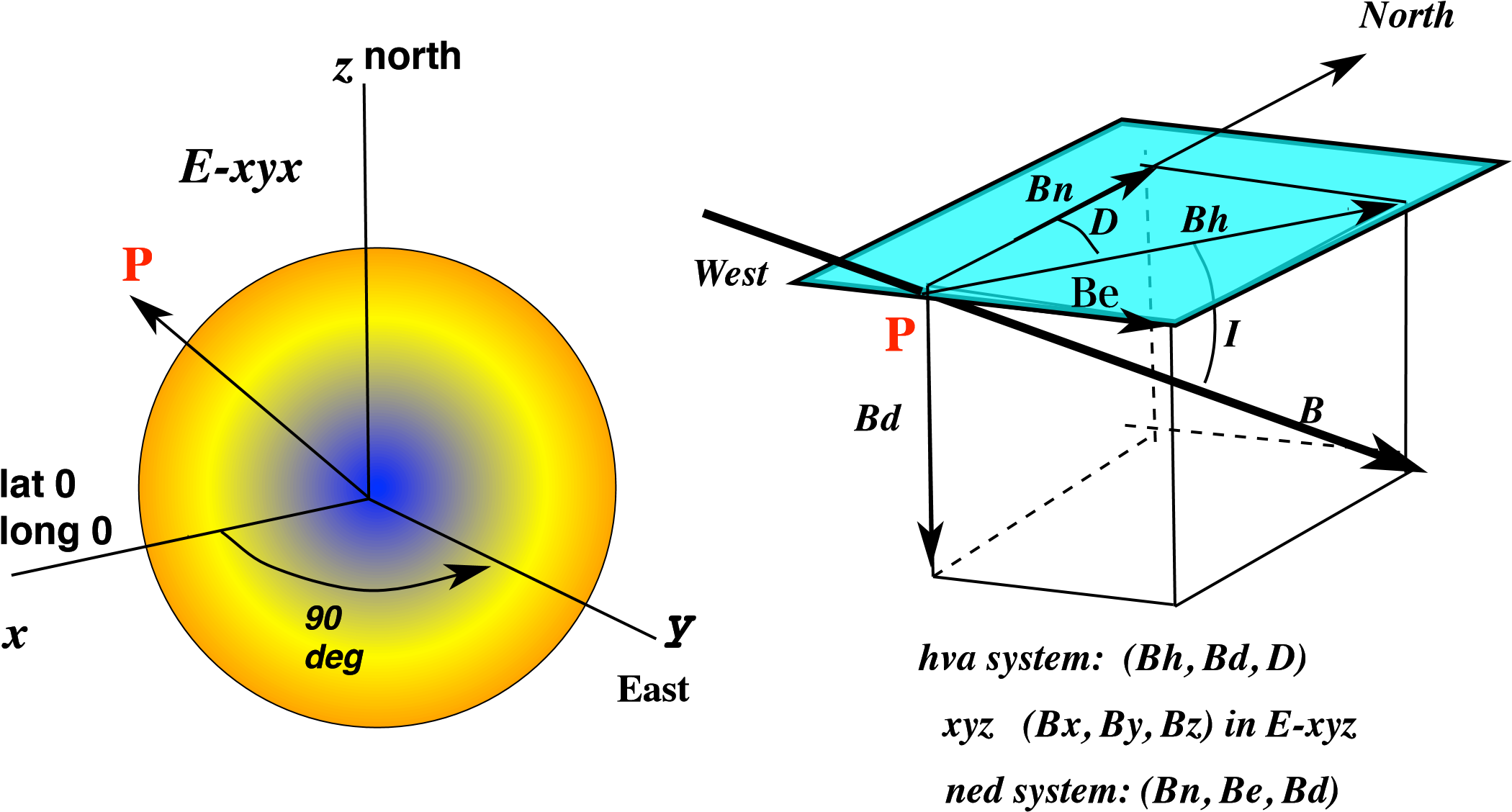
When dealing with the Earth’s magneticfield, it is necessary to understand various coordinate systems, their mutual transformations, and the representation of the three components of the magnetic field vector B.
In understanding the Earth’s magnetic field, it is also worth taking a slight detour to examine the motion of low-energy charged particles influenced by the Earth’s magneticfield.
Fig. 6.2 Left: E-xyz system. Right: Components of the geomagnetic vector B
Earth-centered Cartesian Coordinate System (E-xyz):
Within Cosmos, the position coordinates are expressed using the E-xyz system. It is a coordinate system with the Earth’s center as the origin, the direction of (0,0) latitude and longitude as the x-axis, the north pole direction as the z-axis, and the east direction as the y-axis.
LLH System:
When given the components of the position vector r in the E-xyz system, it may not be intuitive. Therefore, the LLH system is used, where the components are expressed as latitude, longitude, and height (Lat, Long, Height). It is a representation that is more familiar in everyday life. The height is defined as the distance from the mean sealevel defined for each location (in meters), and the latitude and longitude are in degrees.
SPH System:
Although less intuitive than LLH, the spherical coordinate system (SPH) is sometimes used. It consists of the polar angle \(\theta\), azimuthal angle \(\varphi\) (angle measured counterclockwise from the x-axis, with the y-axis at \(\varphi = 90^{o}\) ), and thedistance r from the origin. It can be represented as :math:` (r sin theta cos varphi , r sin theta sin varphi , r cos theta ).
Geomagnetic data is obtained from the International Geomagnetic Reference Field (IGRF), which is revised every five years (expected to be revised in 2025). The data can be found in $LIBLOFT/Data/Geomag/igrf (igrf is a symbolic link to the actual data). If an updated version is installed, the link needs to be updated as well.
There are three ways to represent the magnetic field vector B at a certain point P near the Earth:
* NED: ruby Copy code The standard representation in the IGRF is NED (North, East, Down), where B = (Bn, Be, Bd).
* HVA: Another representation is HVA, where B = (Bh , Bd , D). Here, D is the declination angle between Bh and Bn.
* XYZ: Within Cosmos, the E-xyz system’s orthogonal components (Bx , By , Bz ) are used.
Transformation of Position Coordinates:
The program takes the following form:
#include "Zcoord.h"type(coord)::from! Coordinate to be transformed.type(coord)::to! Transformed coordinate....call ctransCoord2(sys,from,to)...
Here,
sys: represents the target coordinate system which is one of “xyz”, “llh”, or “sph”.
from%sys: contains one of these strings representing the current system.
from%r(1:3): represents the components of the position vector.
to: receives the transformed components. to%sys will contain the same value as ‘sys’. to may be the same varialbe as from.
Conversion of Geomagnetic Vector B
The program takes the following form:
#include "Zcoord.h"#include "Zmagfield.h"character(3)::sys! Desired format of the transformed components: "ned", "hva", or "xyz".type(coord)::pos! Position vector at the location where the magnetic field is given.type(magfield)::fromB! Magnetic field vector to be transformed.! fromB%r(i) for i=1,3 are the components,! fromB%sys is the current format of the components.type(magfield)::toB! Transformed magnetic field vector....call ctransMagTo(sys,pos,fromB,toB)
Note: In the actual program, instead of type(coord)::pos, type(position)::pos is often used, which includes:
#include "Zcoord.h"#include "Zpos.h"type(position)::pospos%xyz%r(i)! i=1,3 are the components of the position vector.pos%xyz%sys! "xyz," "llh," etc.pos%radiallen! Distance from the origin.pos%depth! Thickness in kg/m2 .pos%height! Altitude in meters.pos%colheight! Altitude of the last hadronic interaction in meters.
Exercise to draw magnetic field lines as shown in Fig. 6.1.
- Check if chook.f is linked to chook.f-BfieldLine using ls-l.
- If it is not linked, execute the following commands:
rm chook.f
ln -s chook.f-BfieldLine chook.f
In this example, the structure of the program follows the usual application format. At the stage when the overall initialization is complete (inside chookBgRun in chook.f), it calls the subroutine testBfieldline to perform the desired task and stops and exits upon return. The essential part is the content of testBfieldline.f, so if it is made the main program, chook.f is not necessary, but then it becomes necessary to manually read the IGRF data files. In this case,we take a shortcut to avoid such hassle.
The program testBfieldline.f is included in the last part of chook.f.
The structure of the program to draw magnetic field lines is as follows:
1. Read the starting point’s latitude, longitude, and height from stdin.
2. If the latitude is above 90, exit.
3. Create the position information of the starting point. at that location. Note: The IGRF data is valid near the Earth. At distant points, the accuracy
4. Calculate the B decreases due to factors such as solar wind, and the variable “icon” becomes 1 instead of 0 in the callcgeomag(...,icon) for points over 105 km. This situation occurs when starting from points close to the poles. to the E-xyz system to simultaneously display the magnetic field lines and the Earth.
5. Convert B to the E-xyz system to simultaneously display the magnetic field lines and the Earth
6. Move the current position a short distance “leng” in the direction of B. the northern hemisphere, the direction vector of the magnetic field lines needs to be reversed to draw the lines coming from the southern hemisphere (controlled by the variable “reverse” in the program).
7. If the altitude at that point is below the starting point, exit the loop and proceed to c).
8. The position information consists of three components (x, y, z), but to draw the magnetic field lines with the Earth, it is necessary to output them in the same format as the trace information in FirstKiss, which allows drawing the tracks of particles. The output format of each line is: x y z code K.E charge S. “K.E” (kinetic energy) can be any value, and setting “code” and “charge” to 2 and 1, respectively, will draw positrons, which re represented by default as red lines. “S” represents the accumulated traveled distance divided by the speed of light (\(\beta\) ), but since it is not used, any value can be used. When drawing multiple magnetic field lines, separate the data of each line with two lines of blank space.
9. back to b).
10. c: back to a).
Compilation and Execution:
1. Confirm that the link of chook.f is correct.
2. Execute the following commands: make clean; make. This will create the executable file cosmosxxx (xxx depends on $(ARCH), which can be MacIFC, etc.).
3. The required input data for execution is param-Bfieldline. Specify the year of the geomagnetic field data with YearOfGeomag, but in practice, it is rarely used. Any valid value can be provided.
4. Where to provide the starting point data (LLH)? Since it is set to read from stdin, in the usual case, when the program starts running, you would input the data from the terminal. However, in this case, the execution command ( ./cosmosMacIFC<param-Bfieldline) uses param-Bfieldline as stdin.
5. Therefore, after reading &PARAM and &HPARAM in param-Bfieldline, the program continues to read LLH data. In the example, the longitude is fixed at -112 degrees, and the latitude is given from 70 to 10 degrees in 5-degree increments. The altitude is constant at 30 km.
6. Execute the command: ./cosmos$ARCH<param-Bfieldline>TraceBfield. This will create trace data in the same format as the regular particle tracking.
7. To visualize the data, use the command: dispcosTraceGeomv TraceBfield earth. Note: Currently, geomview is required for displaying the trace. Omitting “earth” will result in no Earth being displayed. If you want to display the shower trace with the Earth, you need to identify the position of the shower and zoom in to see it. Exercise to draw cosmic rays that follow magnetic field lines, as shown in Fig. 6.3.
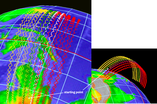
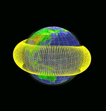
Although we are dealing with UHE-gamma (Ultra-High-Energy Gamma, let’s see what happens to low-energy cosmic rays as they follow the Earth’s magnetic field lines. This movement called “drift and bounce” will be clearly seen in thefollowing animation:
Fig. 6.3 Motion of positive and negative charged particles in the Earth’s magnetic field. Electrons (yellow), positrons (red), protons (white), and antiprotons (green) with the same momentum. They move by alternating between Bounce and Drift. Electrons and antiprotons shift to the east, while positrons and protons shift to the west. Near the starting point, the trajectories of electrons and positrons are obscured by antiprotons and protons, respectively, as their orbits coincide. Protons and antiprotons decay faster. The behavior of Drift is easier to underst and from the left figure.
Compilation and Execution:
Since we will be using chook.f-Bounce, chook.f needs to be linked to it. Note that chook.f itself is not actually used, so attention should be paid to its content.
Use the commands: make clean; make to create the executable program.
The parameter file is “param-Bounce”
+ To fix the injection point, angle etc, we should know the definition of the following input parameters.
Reference observation point: The altitude is the altitude of the lower observation surface plus the OffsetHeight. The default value of OffsetHeight is 0. Latitude and longitude are defined by LatitOfSite and LongitOfSite.
Zenith angle and azimuth angle are determined by sampling using input parameters. Their values are determined by the direction cosine of the vector drawn from the reference observation point to the source (starting point) of the cosmic ray if it traveled in a straight line from the source. This is not the angle at the starting point (it’s the opposite of the vector drawn from the starting point to the observation point).
HeightOfInj: The altitude of the cosmic ray’s starting point. The latitude and longitude of the starting point are determined by the above conditions. If the zenith angle at the starting point is higher than the reference observation point (if the zenith angle is not zero), the value will be smaller at the observation point. The cosine value will be larger.
XaxisFromSouth: South refers to the south along the longitude. When defining the coordinates of a horizontally placed detector, it specifies the angle (in degrees, ranging from \(-360^{o}\) to \(360^{o}\)) that sets the
x-axis from the south in an eastward direction. If the absolute value is greater than \(360^{o}\) (default), the x-axis is aligned with the magnetic east. The z-axis is oriented upward in the vertical direction.
Parameter values in param-Bounce:
Azimuth=(90,90): Cosmic rays incoming from the north.
CosZenith=(0.2,0.2): The cosine of the zenith angle at the observation point is 0.2. The value at the starting point is written to stderr at the end of program execution, which is 0.43 in this case.
BorderHeightH = 5000e3, BorderHeightL = 40e3: Particle tracking is performed within this altitude range. The default value is 0, in which case the tracking range is below the starting point of the 1-ry particle and the lowest observation surface.
The incident cosmic ray is specified in “primary-Bounce”. For example:
Trace=41: Record the particle trace. The coordinate system is E-xyz. Since TraceDir=’./’, the trace will be written as trace1 in the current directory.
With the current settings, the particles are oriented downward, and the magnetic field lines are oriented upward. However, due to the low energy, the particles end up spiraling along the magnetic field lines and moving upward.
Execution: Run the command ./cosmosXXXX<param-Bounce to execute the program. To simulate positrons, protons, or antiprotons, modify the ‘e-’ in primary-Bounce to ‘e+’, ‘p’, or ‘pbar’ (or p~), respectively.
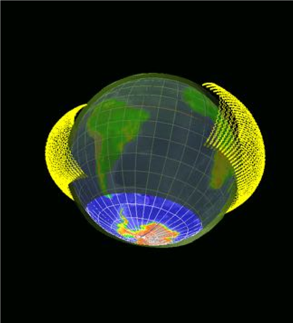
Getting more sidetracked: Let’s explore what happens to cosmic rays as they perform Bounce and Drift motions along the Earth’s outer circumference. We will examine their relationship with the magnetic field and how far they travel.
The first systematic observation to answer such questions was probably conducted by AMS01 (Physics Letters B472, (2000). 215-226; Physics Letters B 484, (2000) 10-22, AMS collaboration).
To reproduce such observations in simulations, it is not enough to manually input the position and momentum of incident particles. It is necessary to track the secondary particles generated by the interaction with the atmosphere by randomly injecting low-energy cosmic rays into the Earth. In that case, considerations must be made for the energy spectra of each type of incident cosmic ray, the location-dependent cutoff due to the Earth’s magnetic field, and other factors.
Fig. 6.4 Example of long-life e- ; AM defines Slong life a flight time > 0.2 s. This example is likely in the 20-second range. It can be seen from the video at that the electron is a descendant of the proton collision.
From observations, AMS01 determined the momentum, origin, and locations where electrons, positrons, protons, and antiprotons penetrate into the atmosphere. They calculated the trajectories and flight times of these particles and obtained distributions as shown below.
The specific simulation method for the corresponding their analysis will be discussed separately. For now, let’s focus on the results.
In the figures, \(\lambda_{m}\) represents the geomagnetic latitude in radians. AMS uses the symbol \(\Theta_{M}\) and radians as units.
Fig. 6.5 Correlation between energy and flight time of e- and e+ . The right side shows the observation results, and the left side shows the Monte Carlo simulation results.
Now let’s move on to the simulation of pair production by UHE-gamma in magnetic fields.
Since we will be using chook.f-Mag, we need to link it with chook.f.
Monitor the name of the first interaction of gamma rays using chookGInt and define a common variable to hold it. Treat it as a module at the beginning of the program.
module modFirstIntInfocharacter(5)::Intname! one of mpair, pair, ...end module modFirstIntInfo
In chookBgRun, call epResetEcrit to reset the critical energy to 81 MeV. The default value in the PDG is approximately 87 MeV, but it seems too large for the calculation of AS size (Ne). Since the hybrid calculation is an approximate calculation, it doesn’t need to be too precise, but 81 MeV is chosen.
In chookBgEvent, initialize the variable that holds the interaction name for each particle to blank. Intname = ‘ ‘.
chookObs does not record the passage of individual particles through the observation surface.
In chookEnEvent, obtain information about the incident particle from cqIncident. Retrieve the direction vector of the source and calculate the zenith angle and azimuthal angle. Use cqFirstIP to determine the position of the first collision point. Use cgeomag to obtain the magnetic field strength (B) at that point, and use cgetBsin to calculate \(B \sin ( \theta )\) (where \(\theta\) s the angle between the particle trajectory and the magnetic field line). Write the event header, including “Bsin”, “Zenith angle at the lowest layer of 1ry”, “Zenith ale at the source of 1ry”, “Azimuthal angle”, “Altitude of the first collision point”, and “Interaction name”.
Next, calculate the AS size at each observation surface. Use “out#” as a marker. Write the “Layer number”, “Vertical depth (g/cm2 )”, “Slant depth”, “Zenith angle”, “Azimuthal angle”, “Bsin”, and “Interaction name”. (Note: Slant depth is calculated by dividing the vertical depth by cos(zenith angle). It introduces significant errors for zenith angles greater than 60 degrees.)
chookGInt: Retrieve the name of the first interaction of gamma rays as IntInfArray(ProcessNo)%process and set never=1 to avoid further calls in this event (In older interface, it was never called for all subsequent events).
Use param-Mag for input parameters. The essential ones are:
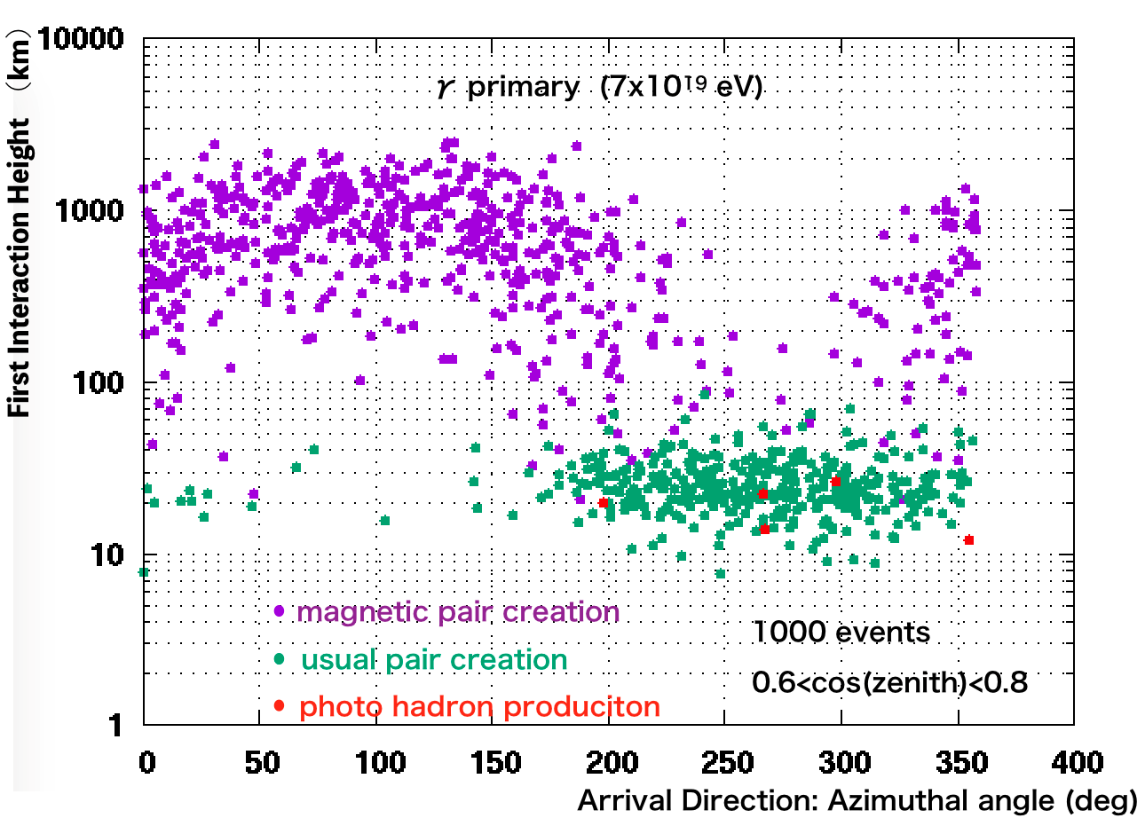
Azimuth = (0.0, 360.0): UHE-gamma arriving from the north should experience the magnetic field effect. Therefore, we only need to investigate the 1ry arriving from approximately \(90 \pm 30\) degrees (where the magnetic field effect is not signfificant) and the south side at approximately \(270 \pm 30\) degrees. However, for the incident 1ry, we consider all azimuth angles and examine the results for each azimuth angle separately.
Zenith angle is set to cos(0.6 ~ 0.8).
Observation altitude is 100 ~ 1000 g/cm2 . The size of Ne is determined using ASDepthList.
Number of events is 1000.
Set Generate to ‘as’ and focus on the size of Hybrid AS. Since low-energy particles are not tracked, ‘em’ is not included.
HeightOfInj = 5000e3: Inject particles from a sufficiently high altitude, which can be considered as vacuum, higher than the usual 100 km.
LatitOfSite = 39.3, LongitOfSite = -112.9: Use the TA site as an example of a mid-latitude site.
LpmEffect = T: LPM effect is included by default.
KEminObs = 8*7.0e5: Consider 1ry with energies above 10^19 eV for Hybrid calculations, so the energy of particles to be tracked (observed) is set to be 700 TeV or higher.
PrimaryFile = ‘primary-Mag’: Specifies the gamma rays and their energies in this file.
HowGeomag = 2: B varies with position.
MagBrem = 2, MagBremEmin = 3e7: Include synchrotron radiation for energies above 3 x 10^16 eV. If MagBrem = 1, gamma rays are not generated, only the energy loss of electrons is considered.
MagPair = 1, MagPairEmin = 2e10: Consider magnetic pair production. The minimum energy is 2 x 10^19 eV.
RatioToE0: Follow hadronic interactions down to per-nucleon energy of RatioToE0 * E0.
WaitRatio = 0.005: Do not connect to the analytic solution of AS until the energy of electrons becomes less than or equal to E0 * WaitRatio.
UpsilonMin = 3e-3: High-energy magnetic effects become significant at \(\Upsilon = \gamma B/B_{c} \approx 0.1\) or higher. Consider synchrotron radiation for values above this threshold (Bc = 4.4 x 10^13 Gauss).
Compile and execute:
make clean; make;
./cosmosXXX < param-Mag > YYYY
From the output, you should be able to create graphs similar to the following (replace YYYY with any desired name).
Fig. 6.6 Correlation between arrival direction and the first interaction altitude. Interactions include magnetic pair creation, regular pair creation, and photo-hadron production. The energy of 1ry is 7 x 10^19 eV.
Fig. 6.7 Ne transition curve. The fluctuations are significantly different depending on the azimuth angle.
Electrons and positrons generated through pair production due to the magnetic field are UHE (Ultra High Energy). Even if they penetrate into the atmosphere, the LPM effect causes significant fluctuations in shower development. However, the fluctuations become smaller because synchrotron radiation occurs in the geomagnetic field. Since the electrons are UHE, classical equations cannot be used to describe synchrotron radiation.
The program uses chook.f-sync, which is a modified version of chook.f called chook.f-Mag that retrieves information about electron synchrotron radiation through subroutine chookEInt in chook.f-sync. Therefore, chook.f is linked to chook.f-sync.
In chookEInt:
if (IntInfArray(ProcessNo).process == “sync”) then
This detects synchrotron radiation and outputs the energy of gamma rays and the energy of the parent electron with the marker sync#.
Since synchrotron radiation can occur multiple times and we want to output all of them, set never = 0.
Use param-sync. The basics are the same as param-Mag. The primary is primary-sync, and we use a slightly lower energy of 5 x 10^19 eV (5e10 GeV).
Azimuth uses the high probability range of 60 ~ 120 degrees where magnetic pair creation occurs. The number of events is reduced to 100.
Fig. 6.8 Correlation between the energy of gamma rays and the energy of the parent electron from synchrotron radiation of electrons generated through magnetic pair creation of UHE-gamma with an energy of 5 x 10^19 eV. As Ee approaches Egamma1ry , Egamma max ~ Ee2 deviates. Examples where more than 10% of the energy is radiated in asingle step can be observed for UHE electrons.