1. What is COSMOS X?
1.1. What can we do with COSMOS X?
COSMOS is a Monte Carlo simulation package to simulate atmospheric air showers produced by high energy particles hitting the earth called Cosmic Rays. Original COSMOS was developed by Prof. Kasahara since 1970’s and continued up to version 8 in 2010’s. The history and references to the older versions are found in the legacy web page [cosmosLegacy] . Together with COSMOS, a detector simulation tool EPICS was also developed by Prof. Kasahara.
Originally COSMOS 9 was developed to integrate the functions of COSMOS and EPICS into a single package. To clarify this extended feature, the new COSMOS is released with a new name COSMOS X, meaning eXtended COSMOS. This document concentrates on the description of the COSMOS X and does not assume any experience of previous COSMOS or EPICS.
Using COSMOS X,
Users can inject any particle available in the list (even unstable particles) with any angle and energy.
Users can define the energy and composition distributions for injection using a simple text file.
Users can switch hadronic interaction models.
Users can access information of individual particle in the shower using a so-called userhook function.
Users can define format and condition of output file(s).
Users can define the electric field and magnetic field.
Users can set non-atmospheric materials such as water and soil.
Users can set non-earth environment such as the Sun.
Through these flexibilities, COSMOS X is suitable for various kinds of cosmic-ray studies.
1.2. Structure
This section describes the outline of the COSMOS X structure for users to have a rough idea of how to use COSMOS X. More practical explanations are found in Section 3 and Section 4.
1.2.1. General structure
When the source package is unpacked, users can find the following subdirectories under the main directory CosmosX_zzzzz/ where zzzzz designates the version number. Usually users need to make their own codes based on (copy, paste and edit) the examples in the Application/ directory.
Cosmos/ Functions to handle air shower development are contained.
Epics/ Functions to handle interactions in material are contained.
LibLoft/ Common functions used for air shower and material are contained.
Scrpt/ Useful scripts are contained.
Application/ Useful sample codes for first usage are contained. Usage of the Application/Example/FirstKiss/ sample is the first step of COSMOS and detail is given in Section 2.4.
1.2.2. User’s flexibility: 3 user control files
In the FirstKiss example, users can find several files to control the simulation, among them users are required to edit three files, primary, param and chook.f.
Primary particles (primary file) This file contains information of the type and energy of the primary particle. In case of the FirstKiss example shown in Listing 1.1 , mono-energetic nitrogen nuclei (isotope with mass number 14 and atomic number 7) with kinetic energy per nucleon (KE/n) 100 GeV are injected. More examples of primary definition are found in the LibLoft/Data/Primary/ directory. Detail description of the primary file is given in Section 3.1.
Simulation setup (param file) This file contains information to setup the simulation. An example (slightly modified) of FirstKiss is shown in Listing 1.2 . The file is a list of parameters with their names and values. This format is called
namelistin FORTRAN and easily read with a single read function. (See FORTRAN textbook for more detail.) Information of the observation site, injection angle, hadronic interaction model and any options are specified in this file. Definitions and formats of all available parameters are listed in Section 3.Simulation control and Output (userhook) You may want to access the information of individual particle during tracking as it is available in the popular detector simulation tools like GEANT. To access the event-by-event information (primary particle, end of shower, etc), micro physics of air shower development, to histogramming the intermediate information and handle the output, and to add any artificial effects, some userhook functions users can define in the chook.f file are very useful.
#
# 'e-' 'MeV' 'KE/n' 'd' 0 / 24-12 Mg 22-11 Na
#
#----------------------------------------------------------
  'iso 14 7' 'GeV' 'KE/n' 'd' 0 /
         100      1.
           0.        0.
&PARAM
LatitOfSite = 30.110000
LongitOfSite = 90.53
YearOfGeomag = 2019.500

DepthList = 3000 4000 6000 10000 0
ASDepthList = 2000 4000.0 6000.0 8000.0 .0 .0

SeedFile = 'Seed'
InitRN = 300798 -3319907
PrimaryFile = 'primary'
CosZenith = (0.9, 0.9)
Azimuth = (0.0,0.0)
HeightOfInj = 100.0e3
DestEventNo = 1000 2

Generate ='em'
ThinSampling = F
IntModel = '"phits" 2.0 "dpmjet3" '
IncMuonPolari = T
KEminObs = 8*100e-6 ! 100 keV
LpmEffect = T
MinPhotoProdE = .152

BaseTime = 10.0
Cont = F
ContFile = ' '
CutOffFile = ' '
Ddelta = 5.00
DeadLine = ' '
DtGMT = 8.00
Freec = T
Hidden = F
Job = ' ' ! This is comment after input data
ObsPlane = 1
OneDim = 0
SkeletonFile = 'SkeletonParam '
SourceDec = 30.0
TimeStructure = T
Trace = 21    ! for display with detector
TraceDir = './'
WaitRatio = 0.01
Within = 99999
Za1ry = 'cos 1'
&END
An example of FirstKiss chook.f in Listing 1.3 shows how to output particle information when a particle arrives at the predefined observation altitude.
#include "cmain.f"
!!! #include "ctemplCeren.f" not needed now
!  *************************************** hook for Beginning of a Run
!  *

      subroutine chookBgRun
      implicit none
#include "Zmanagerp.h"

!            namelist output
      call cwriteParam(ErrorOut, 0)
!            primary information
      call cprintPrim(ErrorOut)
!            observation level information
      call cprintObs(ErrorOut)
      end

!     *********************************** hook for Beginning of  1 event
!     *
      subroutine chookBgEvent
      implicit none
      integer:: num, cumnum
      call cpEventNo(num, cumnum)
      write(*,*) '## ev', num
      end


!     ************************************ hook for observation
!     *
      subroutine chookObs(aTrack, id)
!
      implicit none
#include "Ztrack.h"
#include "Zcode.h"
      integer id  ! input.  1 ==> aTrack is going out from
!                                 outer boundery.
!                           2 ==> reached at an observation level
!                           3 ==> reached at inner boundery.
      type(track):: aTrack
!
!     For id =2, you need not output the z value, because it is always
!     0 (within the computational accuracy).
!
      if(id .eq. 2) then
!     output typical quantities.
            write(*, '(3i3, 1p, 3g15.4)')
     *           aTrack%where,  !  observation level. integer*2.  1 is highest.
     *           aTrack%p%code, !  ptcl code.  integer*2.
     *           aTrack%p%charge, !  charge,  integer*2
     *           aTrack%p%fm%p(4), ! total energy in GeV
     *           aTrack%pos%xyz%r(1), aTrack%pos%xyz%r(2) !  x, y in m
      endif
      end

!    *********************************** hook for end of 1 event
!    * At this moment, 1 event generation has been ended.
!    *
      subroutine chookEnEvent
A schematic explanation of the relationship between these files, functions and system functions is shown in Fig. 1.1. Here cosmosLinuxGfort is the name of executable file in case of the Linux environment.
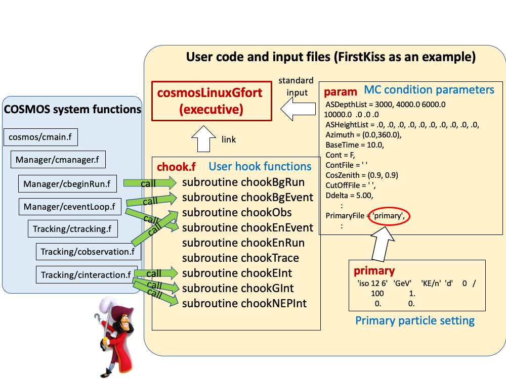
Fig. 1.1 Relation between the COSMOS system functions, userhook functions and parameter files.
Guides to more flexibilities such as arbitrary atmospheric profile, electric field, magnetic field, non-atmospheric material, non-earth sphere are given in Section 4.
1.2.3. What we can not do (now)?
Simulation with arbitrary shape of medium
User code with C++ (in development)